Below is a long post. Understanding it allows you to distinguish between an ordinary software user that program clicking without understanding how it works, and a pipe stress engineer who has an above-average knowledge of what hypothesis underlies the strength of materials. If you belong to the second group, then this post is for you.
PRINCIPAL STRESSES AND STRESS HYPOTHESES
Let us imagine a material element subjected to tension as shown in the figure below. The a – a plane is directed at an angle alpha to the direction of the force F acting on the plane A, generating a tensile stress S. The force F can be resolved into two components: Fn – normal and Fs – tangent to the plane a – a. These components cause normal stresses sigma and tangential stresses theta with values described by the formulas below:
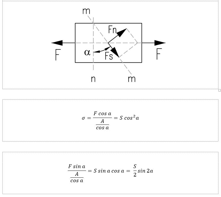
It is obvious that for a constant value of the force F, the normal and tangential stresses depend only on the angle of inclination of the plane. The maximum tangential stress theta will be for sin 2 alfa = 1 (which corresponds to the angle a = 450) half the value of the tensile stress of the sample. The maximum of the normal stress sigma will of course occur for the angle alpha = 00, and its minimum for angle alpha = 900. Stresses in such planes are characterized by the absence of a tangential component and are called principal stress.
Traditionally, principal stresses have been determined using a series of simple constructions from analytical geometry called Mohr's circle, an example of which is given below.
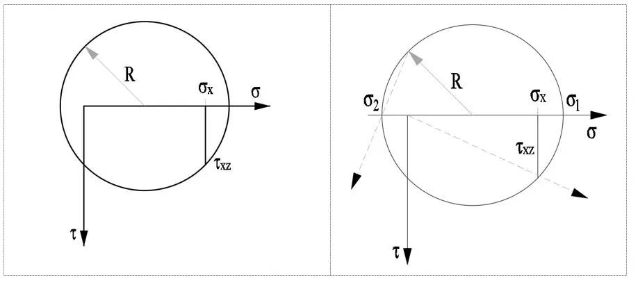
Let us assume that the normal stress sigmax and shear thetaxz are greater than zero and can be shown in the sigma-tetea coordinate system below. We put the value of the normal stress sigmax on the s-axis, and at its end the tangential stress value thetaxz.
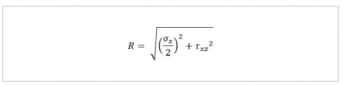
We draw a circle of radius R, the beginning of which is half the value of the normal stress sigmax. We determine the maximum and minimum principal stresses, where the circle intersects at the points of zero tangential stress theta. In the last step, we determine the directions of their action.
Principal stresses (here sigma1, sigma2, sigma3) are the starting point for the two hypotheses used in the pipeline calculations.
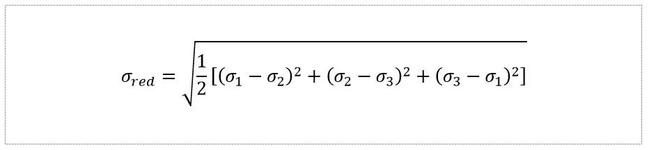
The first one is the hypothesis of the specific work of purely shear deformation formulated and published in 1904 by the outstanding Polish professor M.T Hubera (1872-1950) more widely known as the hypothesis R. Misesa (1883-1953), who published it only nine (!) years later, in 1913. Both were under the resumption of the same ruler, Franz Joseph I, except that the former was a Pole born in a tiny town in Podhale, and the latter an Austrian living in the capital of the Empire in Vienna. Whether this was the theft of the century that the Austrian aristocrat got away with is difficult to decide now. However, there was something to fight for, because the hypothesis of the specific work of purely shear deformation, which was the crowning achievement of many European scientists throughout the 19th century, is the same as Maxwell's four equations for our electromagnetic civilization. This is the fudamental basis of the science of strength of materials.
The general form of the equation for the triaxial stress state is as follows:
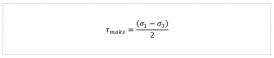
The second hypothesis, the Tresca-Coloumba greatest tangential stress hypothesis, which postulates that the material's stress is determined by the material's achievement of a critical tangential stress. For simple tension, this value is half of the tensile stress. For a triaxial stress state, the stress value is:
PRACTICAL USE OF THE MOHR CIRCLE
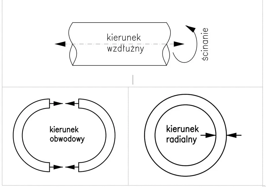
Let us assume a local coordinate system with the names characteristic of a pipeline system: longitudinal stress (stress along the pipe), circumferential stress (or circumferential stress on the circumference) and radial stress passing through the pipe wall. They are shown in the figure below.
In the next step, a cube was isolated from the pipe wall and the principal stresses were applied. We thus have the stresses: longitudinal sigmaL, shear theta , peripheral sigmaH and radial sigmaR.
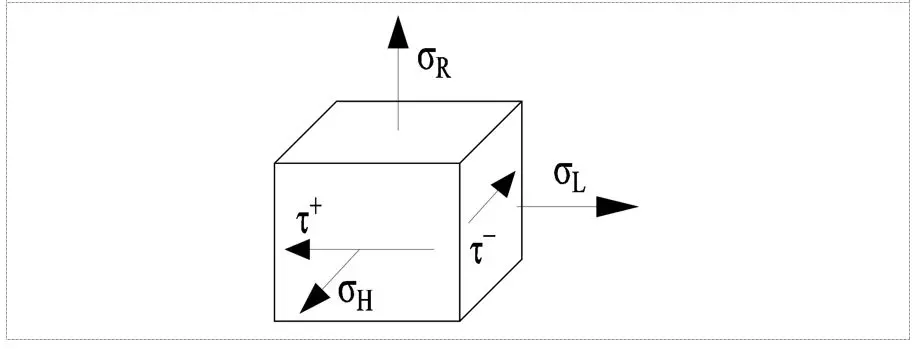
In the next step we define the above stresses, which are the result of displacement, mainly thermal, and not internal pressure:
- Longitudinal: force / cross-sectional area and/or bending moment / bending modulus of cross-sectional strength
- on the wall thickness: negligible for thin walls
- Radial: Zero on the outer surface
- Shear: Shear force / 2 x shear section modulus.
From the above table it can be seen that if the cause is displacement, only the longitudinal and shear stresses are different from zero. Additionally, they are balanced because the system remains at rest.
After being cut by a plane, the system remains in equilibrium. To determine the stresses in the new plane, we can use Mohr's circle construction.
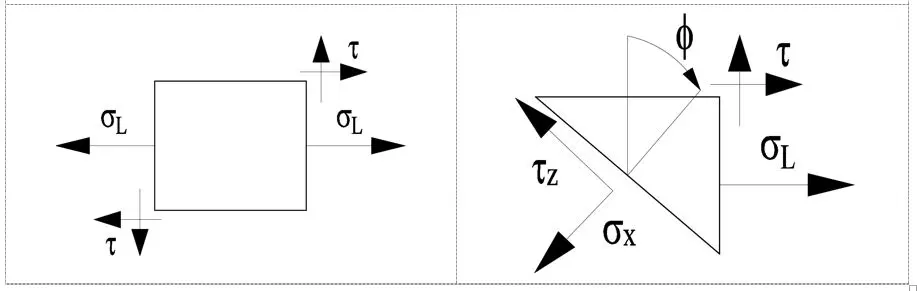
As we know, the principal stress occurs when the shear stresses are equal to zero. The circle intersects the ordinate axis at two such points, which are marked with stress pairs, at which the theta stress is equal to zero. Any angle phi of intersection with the plane can be found from the scheme below, and then the normal and shear stresses can be determined graphically.
The principal stresses in the displacement loaded pipe occur at three points from S1 to S3:
- S1 with the highest value corresponds to stretching
- S2 is equal to zero, which corresponds to radials
- S3 corresponds to compression
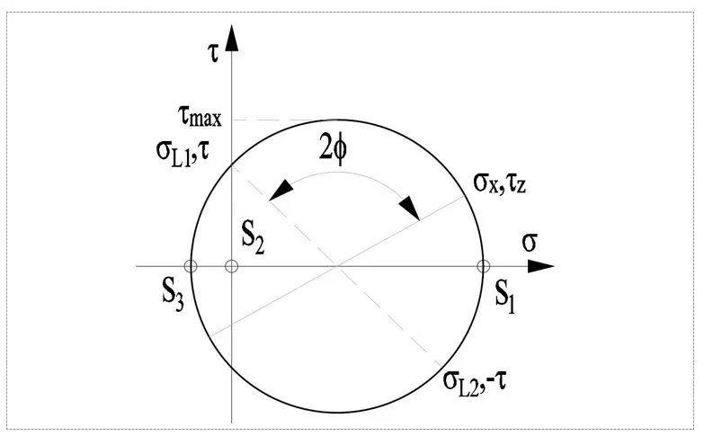
From Mohr's circle, the maximum shear stress can be determined, the value of which can be determined by the simple formula below. In design standards, e.g. ASME B31.3, this is the strength limit of the material.
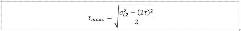
The above formula can be compared with the known standard dependence, which turns out to be identical in principle. The topic of standard calculations will be developed in the next thread