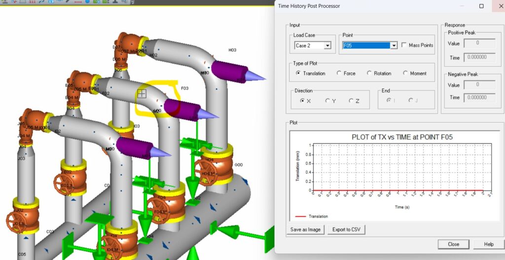
Time history analysis is the most advanced dynamic analysis method, allowing us to study a pipeline's response to loads that vary over time. Unlike static analysis, where the force is constant, we examine what happens to the system second by second or millisecond by millisecond. It's like recording a video of the pipeline's behavior instead of taking a single photo.
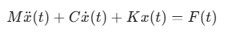
The most commonly used method is modal superposition. The program first calculates the natural vibration modes (frequencies) and then "assembles" the response of the entire system based on how individual modes respond to a given excitation over time. The essence of the analysis is to solve the following equation, where the following matrices are: M for mass, C for damping, K for stiffness, and F for the excitation force vector.
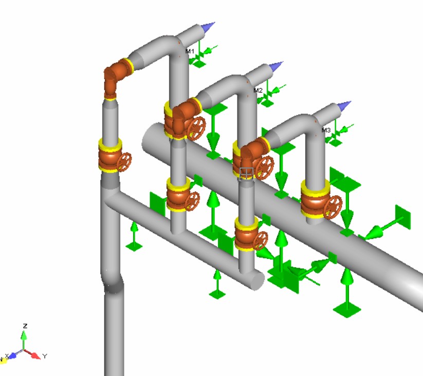
When is time history used? We use this method to simulate short-term, rapid events. Below is an example of analyzing a bank of 4x6-inch natural gas safety valves at pressures of 6.4 MPa/1.15 MPa. Determining the force profile:
- T=0.00 s: Force = 0 Valve closed
- T=0.01 s: Force = 35 kN
- T=0.50 s: Force = 35 kN
- T=0.51 s: Force=0 Valve closing
The AutoPipe model shows the following static analysis results. Ideally, 100% of the B31.3 code stress
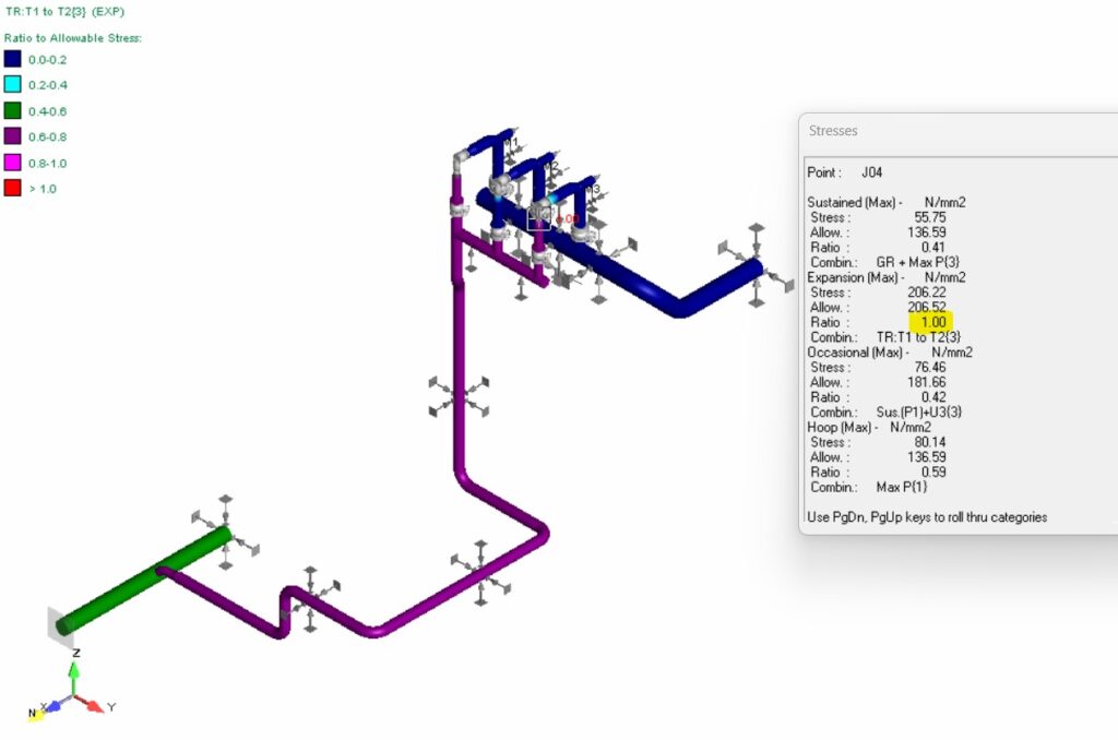
A force of 35 kN is applied to the centers of the arches. This force is absorbed by the triunion supports with the LS function.
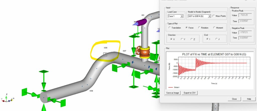
To demonstrate how the presence or absence of the first support downstream of the PSV valve affects the dynamic results, it was removed from the first set from the top. The absence of the support causes the displacement to dampen the oscillations.
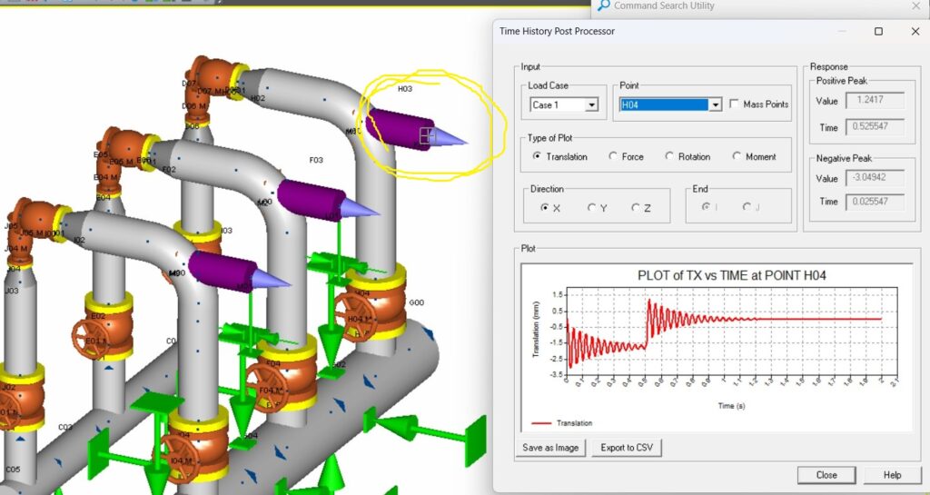
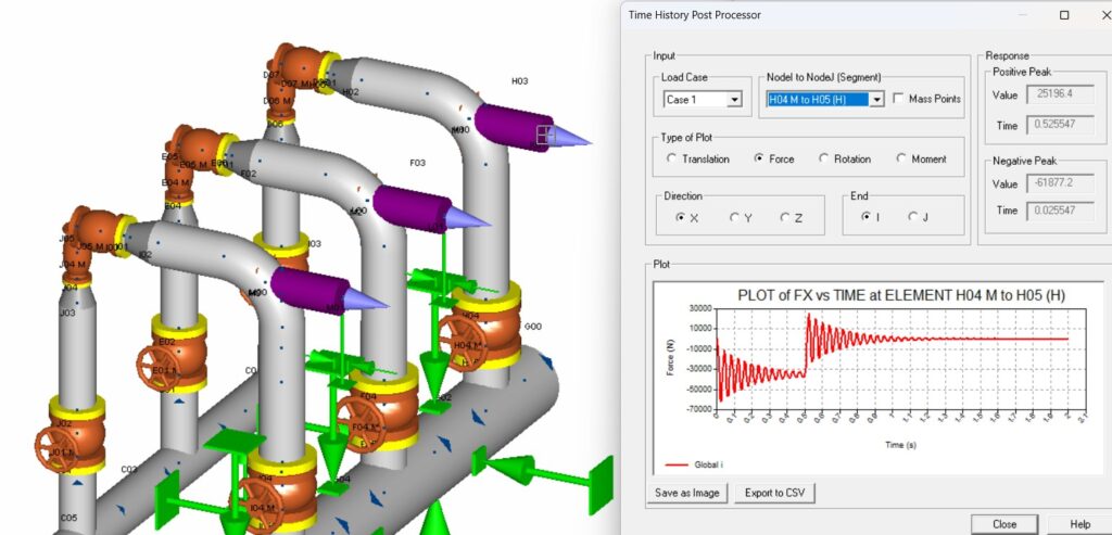
Also, very large force oscillations, which significantly exceed the recoil force of 35 kN, can now be calculated as the actual DLF factor of 61 / 35 = 1.85. This shows that frequently assuming a maximum DLF value of 2.0 can sometimes be justified. In this case, it can be justified by the support failure scenario.
It's interesting to see how the oscillations develop further along the pipeline. For example, at the first elbow of the collector, the force is significantly lower, only 18 kN.
For comparison, in a situation where the support is working properly, the pipeline and the support are so stiff that no oscillation occurs.